Over the course of my summer break in 2020, I completed a System Identificaton internship with Kitty Hawk’s Heaviside team. I developed a complete System ID toolkit for all phases of VTOL flight (hover, transition & forward flight). I wrote all of my code in MATLAB and based my work on SIDPAC

I performed system ID in both the frequency and time domains to model our aircraft’s aerodynamic stability/control derivatives and come up with the aircraft’s transfer functions for use in our controller’s inverse plant model.
I wrote four different simulation models, including one with non-linear and time-variant dynamics, to validate the flight test data and system ID tools.
All in all, I developed over 100 scripts and functions to integrate system ID in our workflow, and wrote 11 documents covering the theory behind my work; all during my 10 week internship.

Since sharing the system ID work I performed while working for Kitty Hawk would be in violation of my NDA, I’d like to provide a brief overview of system ID and its uses instead.

A Brief Overview of System ID and How It Works

What is System ID and Why is it Important?

There are three fundamental aircraft dynamics and control problems:

Simulation: given the input u and the system model s, determine the output y
Control: given the system model S amd the output y, find the input u
System Identification: given the input u and the output y, find the system model S

In short, system identification involves the numerical determination of a dynamic system’s properties from a record of its response to certain inputs in the time domain. For aircraft specifically, flight test recordings are used as a basis to model dynamic behavior.

For aircraft, system ID involves performing operations on measured flight data to come up with:

Aerodynamic coefficients to characterize performance (& control)
Transfer functions to characterize control

System ID yields information crucial to control design: you can’t design a controller to control something without having a good idea of what you’re trying to control!

System ID is also extremely useful for the validation and calibration of design and modelling tools. By comparing the expected performance and control of your aicraft to your aircraft’s actual, measured performance and control, you can learn a lot about your modelling tools!

So then: where does system ID sit in the research and development feedback loop? 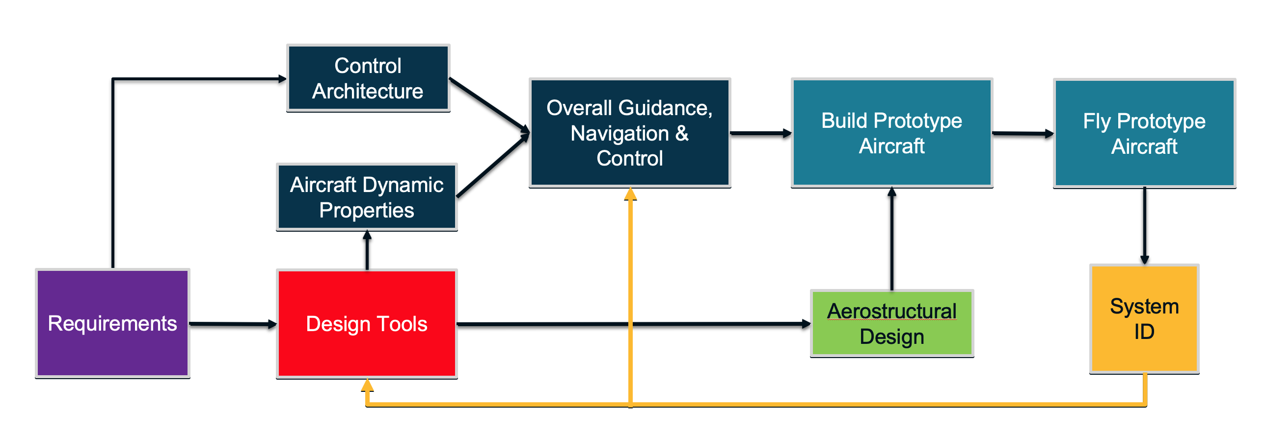System ID in R&D Figure 1: Where System ID Sits in the R&D Feedback Loop

How Does System ID Actually Work?

Many different techniques exist to perform system ID, though system ID methods are largely separated into two categories according to the domains in which they operate. Some tools operate on data in the time domain, and others operate on data collected in the time domain and transformed into the frequency domain.

One of the most difficult parts of the system ID process is verifying that your identified models accurately represent the aircraft’s true dynamic behavior. Each time a model is identified, a verification procedure must be used to confirm that the identified model yields responses very similar fashion to those of the actual aircraft. To complete this verification step, measured responses to measured inputs are compared to the identified plant’s simulated responses to measured inputs.

The flow chart below illustrates the various stages of the system ID process along with the inputs and outputs of time domain and frequency domain system ID methods.

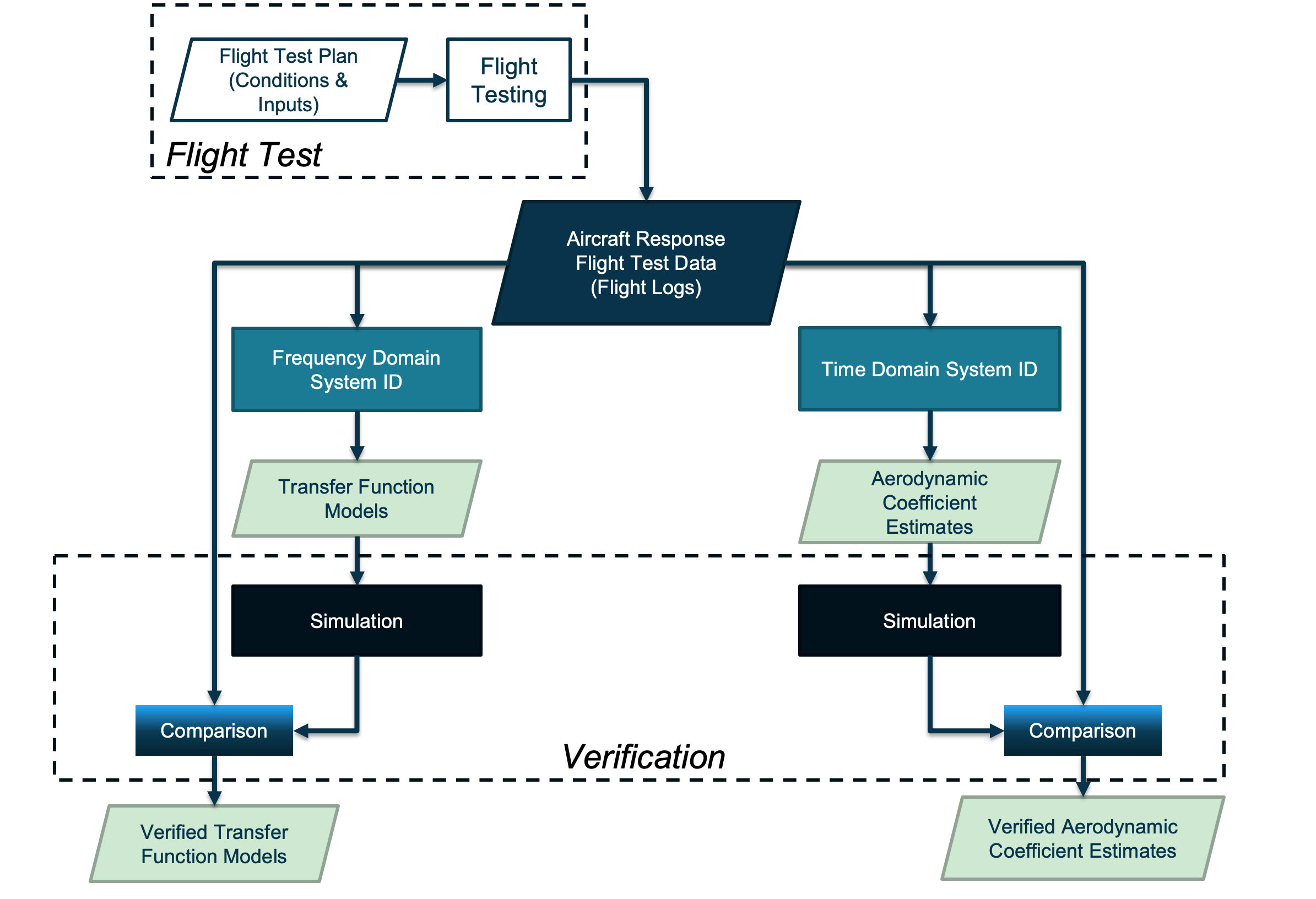Time Dom Freq Dom Figure 2: System ID Process Flow Chart

System ID In the Time Domain Using Linear Least-Squares

Time domain system ID methods are used primarily to estimate aerodynamic stability and control coefficients (aerodynamic derivatives) using linear least-squares regression. As their name suggests, stability derivatives represent the rate of change of a force or moment quantity with respect to some perturbation quantity.

One simple example of a stability derivative is the lift curve slope, or how the aicraft’s lift coefficient (force coefficient) changes with respect to angle of attack (perturbed variable).

In order to identify an aircraft’s lift curve slope from flight test data, one must naturally evaluate the rate of change of lift coefficent with respect to angle of attack change. This can be done very efficiently using linear least squares in the time domain!

Linear least squares is a very powerful method used to approximate linear functions from several sets of data. Imagine a case where we wish to characterize our aircraft’s lift properties by identifying its lift coefficient derivatives from the recordings of a longitudinal maneuver (like an elevator step input), using linear least squares. First, we must select our regressors, the quantity with which we’d like to take the derivative of lift coefficent.

In this case, we can choose our regressors to be:

Angle of attack
Pitch angle
Elevator control deflection

Now, we can use linear least squares to estimate the rate of change of lift coefficient with respect to our regressors, leaving us with our identified derivatives! Linear least squares can also be used to calculate the steady-state value, or “bias” of a quantity, such as steady-state lift or drag. Each parameter estimate’s constant part is appended to the bias term, which represents the steady-state (trim) value of the coefficient.

It is important to note, however, that time-domain system identification methods like the one outlined above are only useful for aircraft in forward flight. In the case of a vertical takeoff or landing (VTOL) aircraft, the scope of this type of identification is actually limited, since the aircraft spends a significant fraction of its time outside of the forward flight regime.

The figures below illustrate the result of linear least squares system identification on the simulated response of an aircraft to a 3-2-1-1 step-type input.

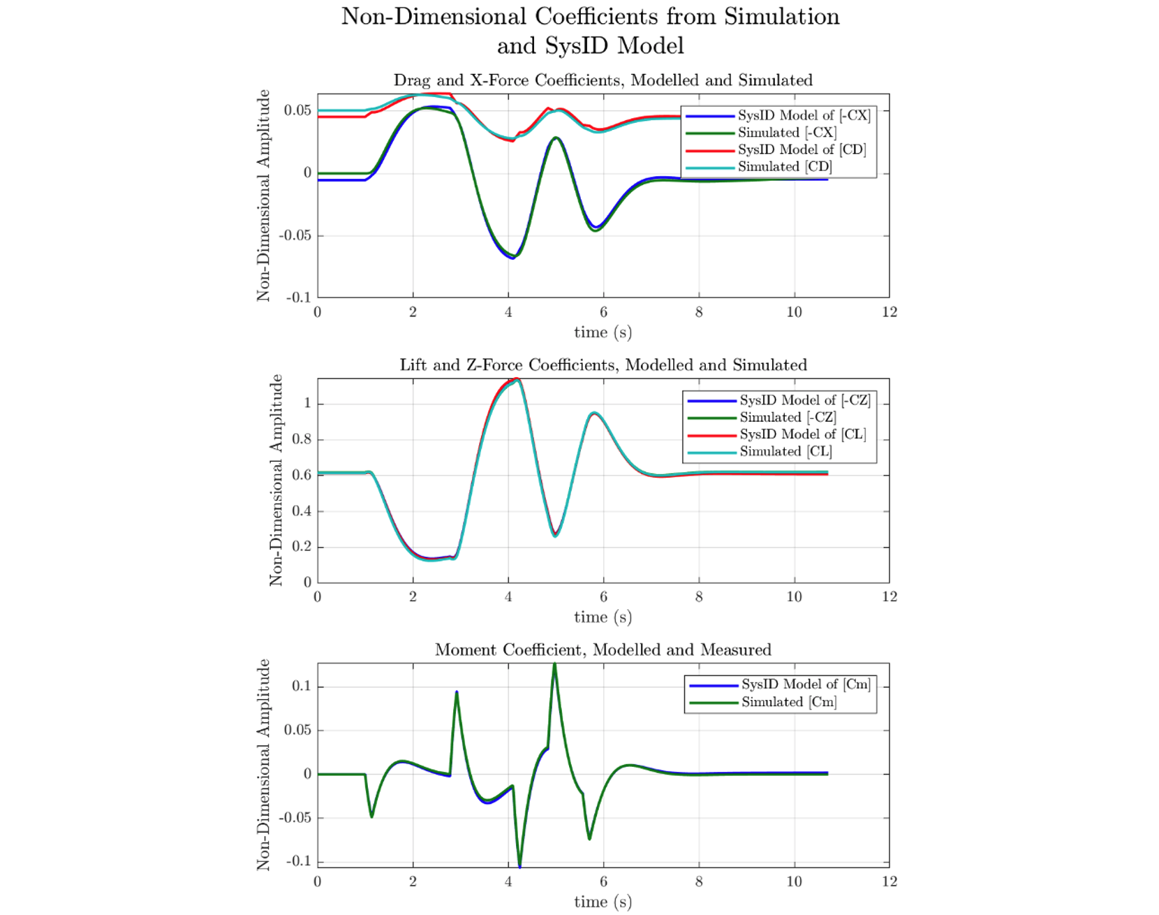Figure 3: Example of Time-Domain System ID

System ID in the Frequency Domain

Whereas time-domain system ID is useless outside of the forward flight regime, system ID can be performed in the frequency domain to determine an aircraft’s transfer functions in any phase of VTOL flight. Further, transfer function system ID is of utmost importance in control system design and plant modelling.

In order to successfully model an aircraft’s behavior using frequency domain methods, sufficent frequency content must be available in the aircraft’s flight recordings. This is a limiting factor of this type of system ID, and special flight test maneuvers (like frequency sweeps and multisines) must be executed in order to get the necessary frequency content. If available flight data does not contain the necessary frequency content, frequency domain system ID is impossible, since without sufficient information on how an aircraft responds to inputs in the frequency domain, it is impossible to identify the system in the frequency domain!

The general frequency domain system ID procedure for estimating transfer function is as follows. First, the time-domain flight data must be converted to the frequency domain using a discrete Fourier transform. Next, the transfer function numerator and denominator orders must be specified in order to build up a model with a set of parameters to match to the measured frequency responses. Once a model is set up, equation-error modelling can be used to estimate the value of each parameter within the transfer function.

For example, if we have a numerator of order 3 and a denominator of order 4 (as is the case for the transfer function of angle of attack with respect to elevator input), like the one below: ade

Then we must identify the value of 9 parameters: 4 for the numerator and 5 for the denominator. ade

Estimation of these parameter is generally completed using one of two methods in the frequency domain: equation-error modelling or output-error modelling (depending on how much measurement error exists in your data). I won’t go into detail on how these methods work, but you can learn more about equation-error modelling by reading this paper, and about output-error modelling by reading this MATLAB documentation.

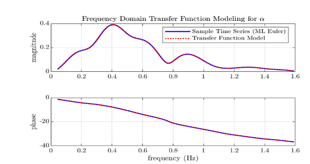
An example of transfer function estimation using equation-error modelling and the same data as in Figure 3 is shown below.

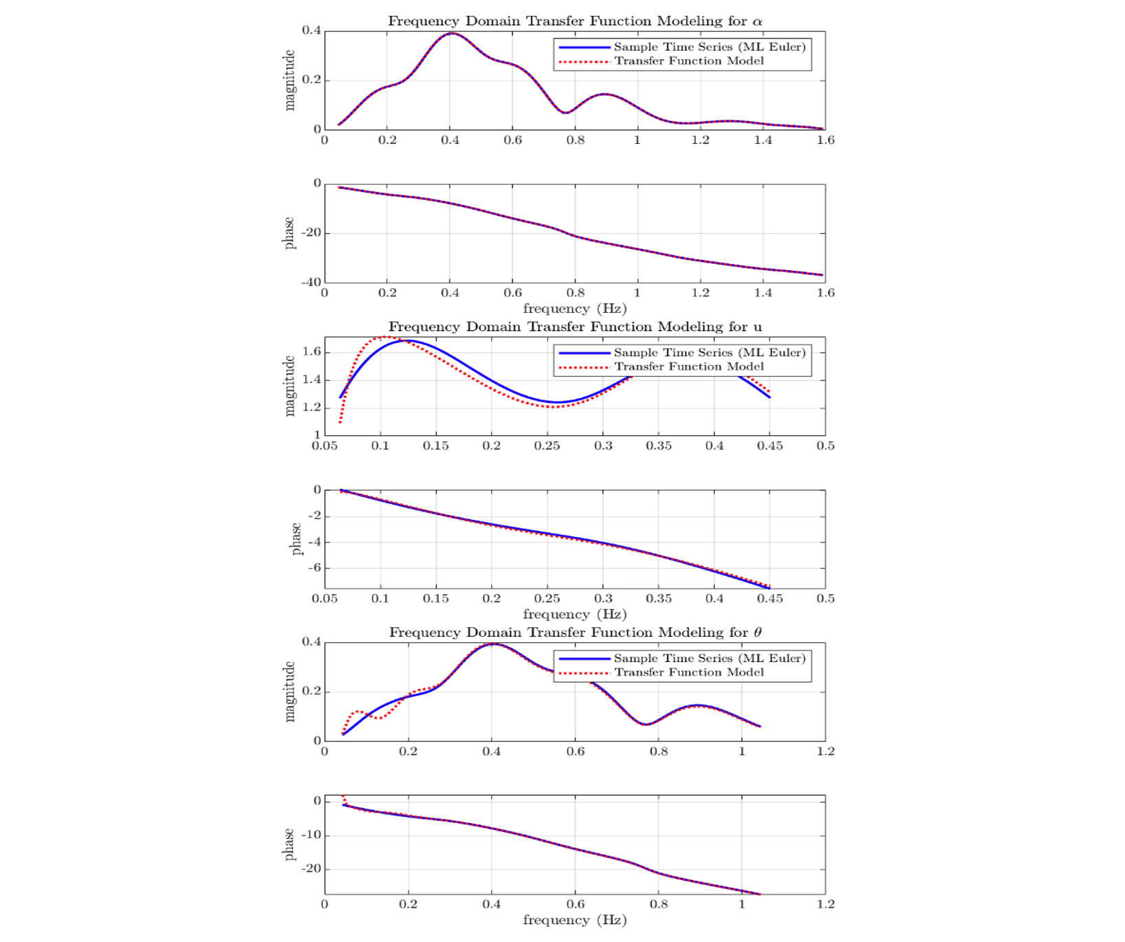ade Figure 4: Frequency-Domain Modelling of a 3-2-1-1 Longitudinal Input Using the Equation-Error Technique